Do you need SEO tools for keyword research? Perhaps you’re looking for a convenient way to track the effectiveness of your SEO efforts.
Google Sheets is a free and cloud-based tool that you can use to collect and organize SEO data. However, to make optimal use of this robust resource, you need to understand how Google Sheets formulas work.
In this blog post, our team at Connective takes an in-depth look at useful Google Sheet formulas for SEO. These basic formulas can save you valuable time and resources.
The best Google Sheets formulas to import data and calculate search volume
The sections below discuss Google Sheets formulas for search engine optimization. Keep reading to learn more. You can also check and copy THIS SHEET to guide you on the formulas that were used here.
ARRAYFORMULA
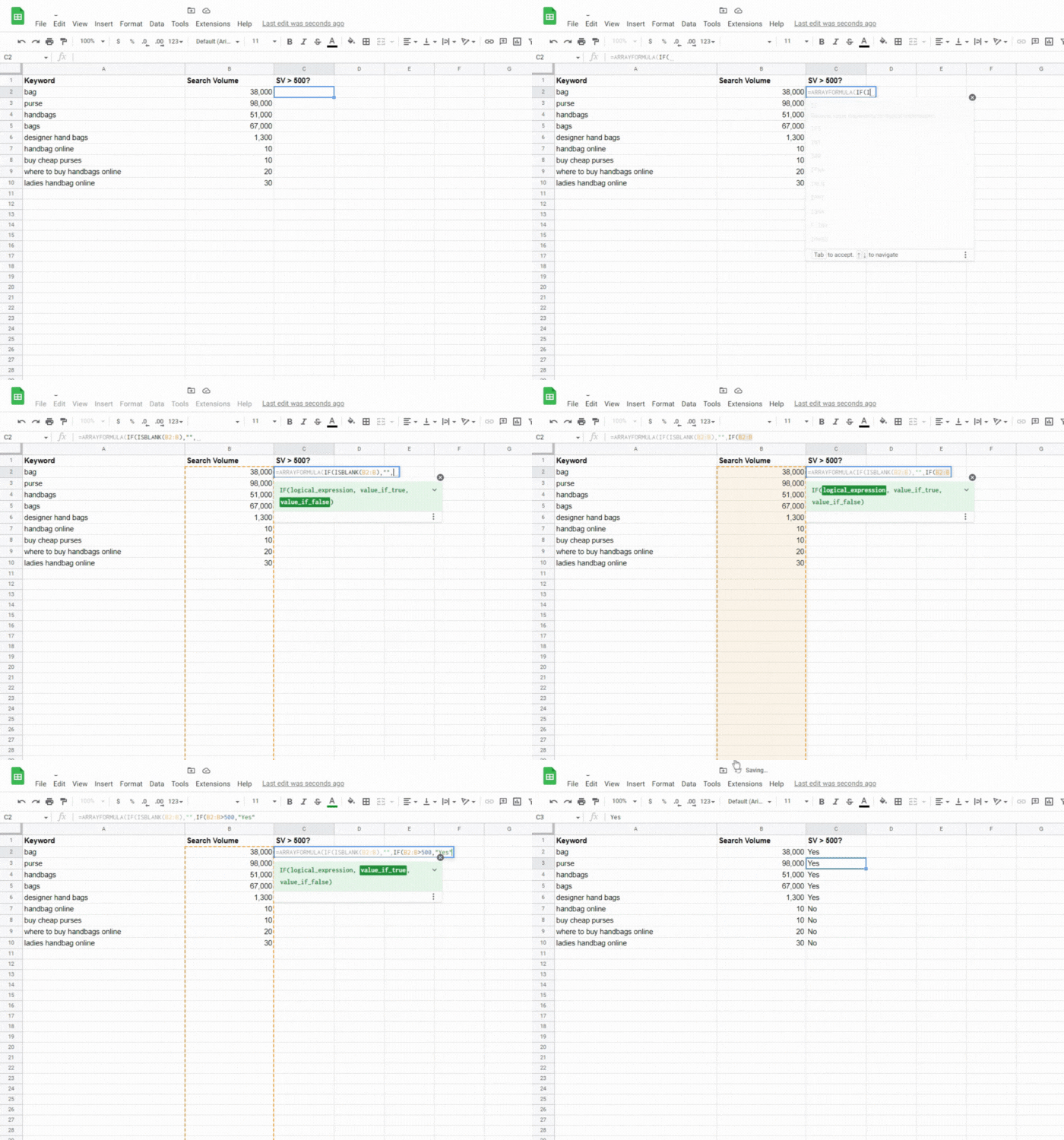
An ARRAYFORMULA returns values in multiple rows or columns. In other words, you can write a formula once, then apply it to an entire row or column.
You can combine an ARRAYFORMULA with an IF formula to determine which keywords meet your visit threshold, for example:
=ARRAYFORMULA(IF(C2:C100>500, “Yes”,”No”))
Paste this formula into the first row of your range. For example, if column C lists the traffic volume for each keyword, you can paste this formula into cell D2. Column D will automatically populate with Yes/No results.
CONCATENATE
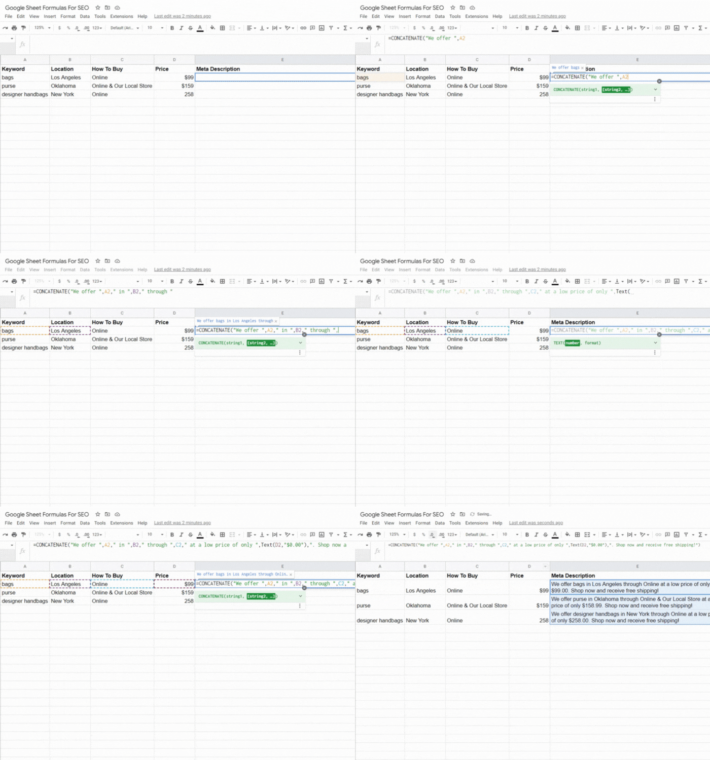
The CONCATENATE formula lets you combine the content of multiple cells into one cell. For example, suppose you want to combine a name in cell A2 with a surname in cell B2. In this case, you can create the following CONCATENATE formula in cell C2:
=CONCATENATE(A2, “ “, B2)
The formula leaves no space between the content from the two cells, and you need to add this space in quotation marks. Instead of a space, you can add text, numbers, or special characters to make the data easier to read.
The CONCATENATE function is helpful if you want to create meta descriptions or title tags in bulk.
For example:
=CONCATENATE(“We offer “,B2,” in “,D2,” by “,C2,” at a low price of only “,E2,”. Shop now and receive free shipping!”)
COUNTIF
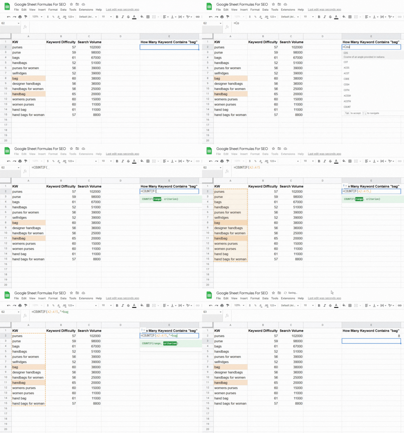
With the COUNTIF formula, you can quickly calculate the number of cells that meet specified criteria. For example, if you have a data set consisting of keywords, you can use this function to determine how many location-specific keywords are in your list. The formula for this function is:
=COUNTIF(range,”specific value”)
For example:
=COUNTIF(C2:C100, “MARYLAND”)
You can also use this function to determine how many cells in your data set meet a specific criterion. For example, if you want to find out how many keywords have a search volume of more than 500, you can use the following formula:
=COUNTIF(C2:C100, “>500”)
IF
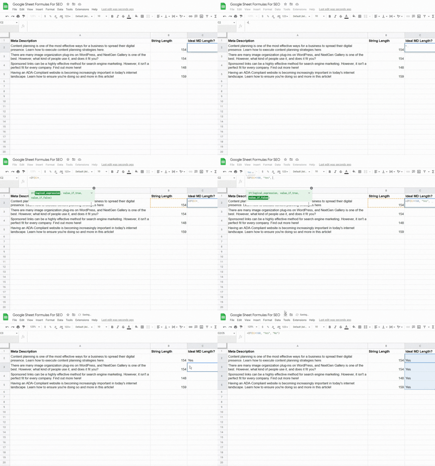
With the IF function, you can test if a cell within a range meets specific requirements with conditional formatting. In this case, the result is either TRUE or FALSE.
The IF formula syntax:
=IF(logical_expression, value_if_true, value_if_false)
The logical expression is a yes-or-no question that uses operators such as =, <, >, >=, <=, and <>.
The values are the references that the function returns, depending on whether the logical result is TRUE or FALSE. Examples of these values include Yes, No, True, or False.
In an SEO context, you can use this function to quickly gauge whether a keyword’s estimated search traffic volumes meet certain conditions.
IFERROR
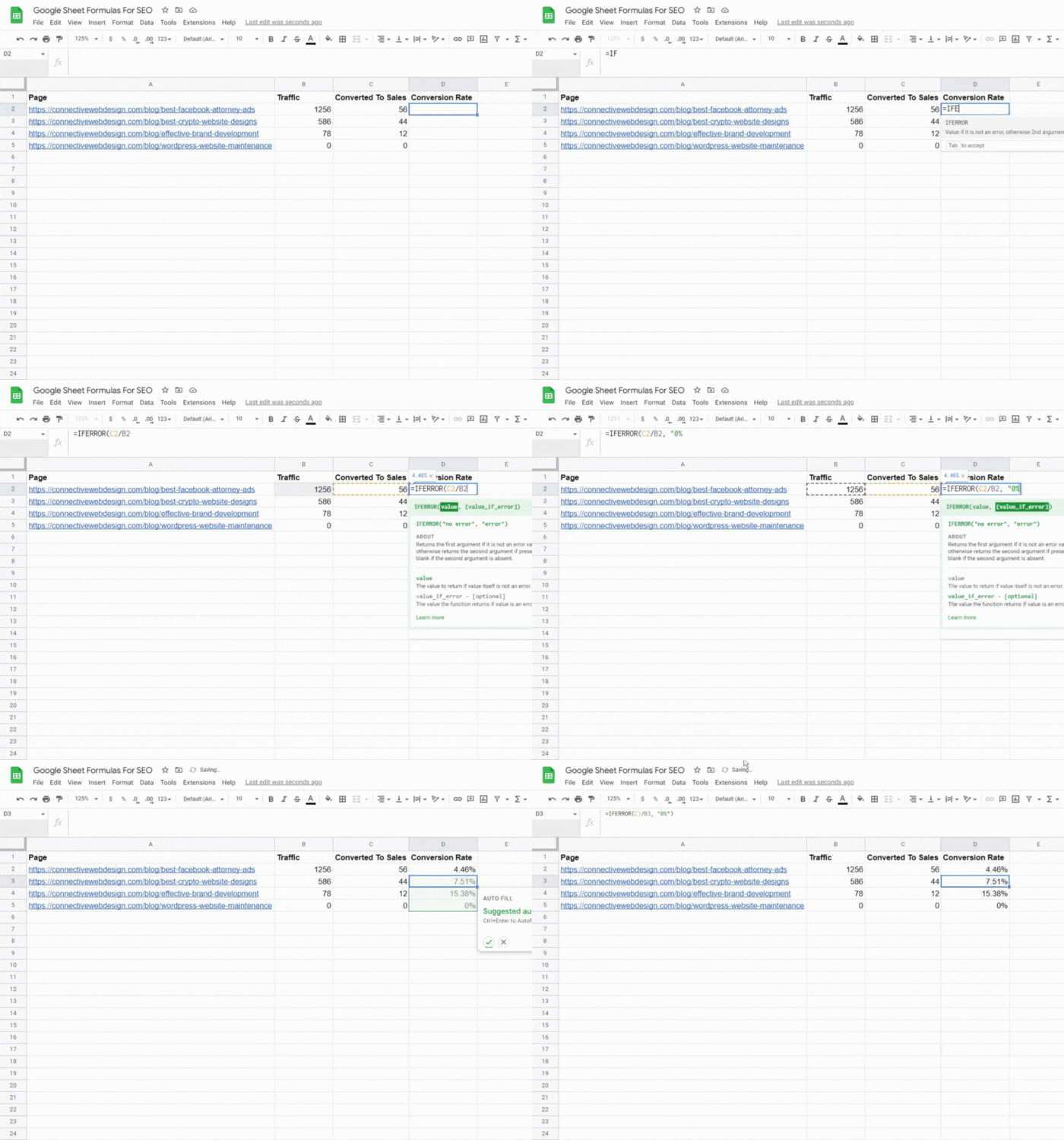
Sometimes, you might encounter an error prompt or non-numerical value, such as #VALUE!, #DIV/O, or #ERROR! This error prompt default value can show up if you use an unknown range or try to divide by zero.
These error prompts are problematic if you want to use the cells to calculate a formula result, and they can make your spreadsheet look untidy.
With the IFERROR formula, you can replace the error prompts with your own default value. You can also choose to leave the cell blank.
The IFERROR syntax:
=IFERROR(original_formula, value_if_error)
For example, suppose your formula calculates a conversion rate by dividing the number of sales by your traffic volume. However, if you have had no traffic, the formula will divide by zero and get an error prompt. To replace the error message with a certain value, for example, “No traffic,” you can use the following formula:
=IFERROR(C2/D2*100), ”No traffic”)
IMPORTRANGE
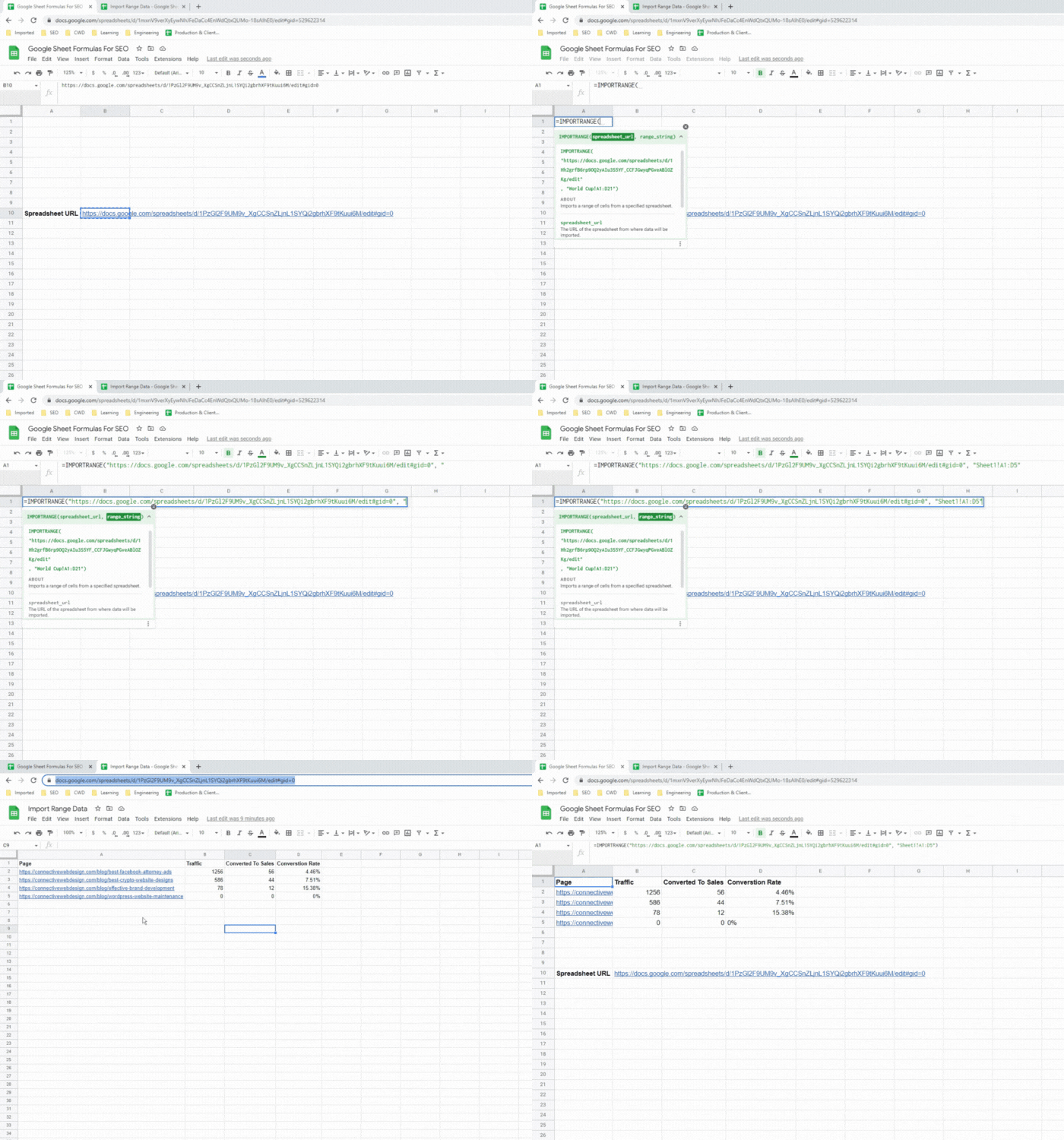
If you are using multiple Google Sheets files when working on a project, some ranges in your sheets might contain the same data, which means plenty of copying and pasting. With the IMPORTRANGE formula, you can import cell data from a master spreadsheet to create client-facing sheets while saving valuable time.
The IMPORTRANGE syntax:
=IMPORTRANGE(spreadsheet_URL, range_string)
This formula needs the URL of the master spreadsheet from which you are importing the data range. You can open this file, copy the URL from the address bar, and paste it into your formula.
After creating the formula, you might get a #REF! error because the spreadsheet needs permission to pull data. Hover your cursor over this error to get the blue “Allow access” button.
IMPORTXML
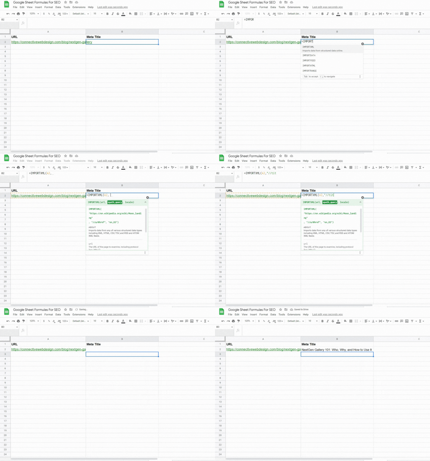
The IMPORTXML function is one of the most useful Google Sheets formulas for SEO. Using this function, you can quickly scrape data from the internet, such as a competitor’s onsite SEO elements, and import them directly into your Google Sheets.
The IMPORTXML syntax:
=IMPORTXML(URL, xpath_query)
In this formula, the URL is the web page address from which you are pulling the information. This value must include the protocol (HTTP:// or HTTPS://).
You should also include the URL in quotation marks. If a cell in your Google Sheets file contains the URL, your IMPORTXML formula can reference this cell.
The Xpath query depends on the structured data types you want to scrape. For example, the Xpath for extracting a meta description is “//meta[@name=’description’]/@content”.
Other examples of Xpaths you can use to extract data include:
- All internal links: “//a[contains(@href, ‘example.com’)]/@href”
- All external links: “//a[not(contains(@href, ‘example.com’))]/@href”
- All links: “//@href”
- The page title: “//title”
ISBLANK
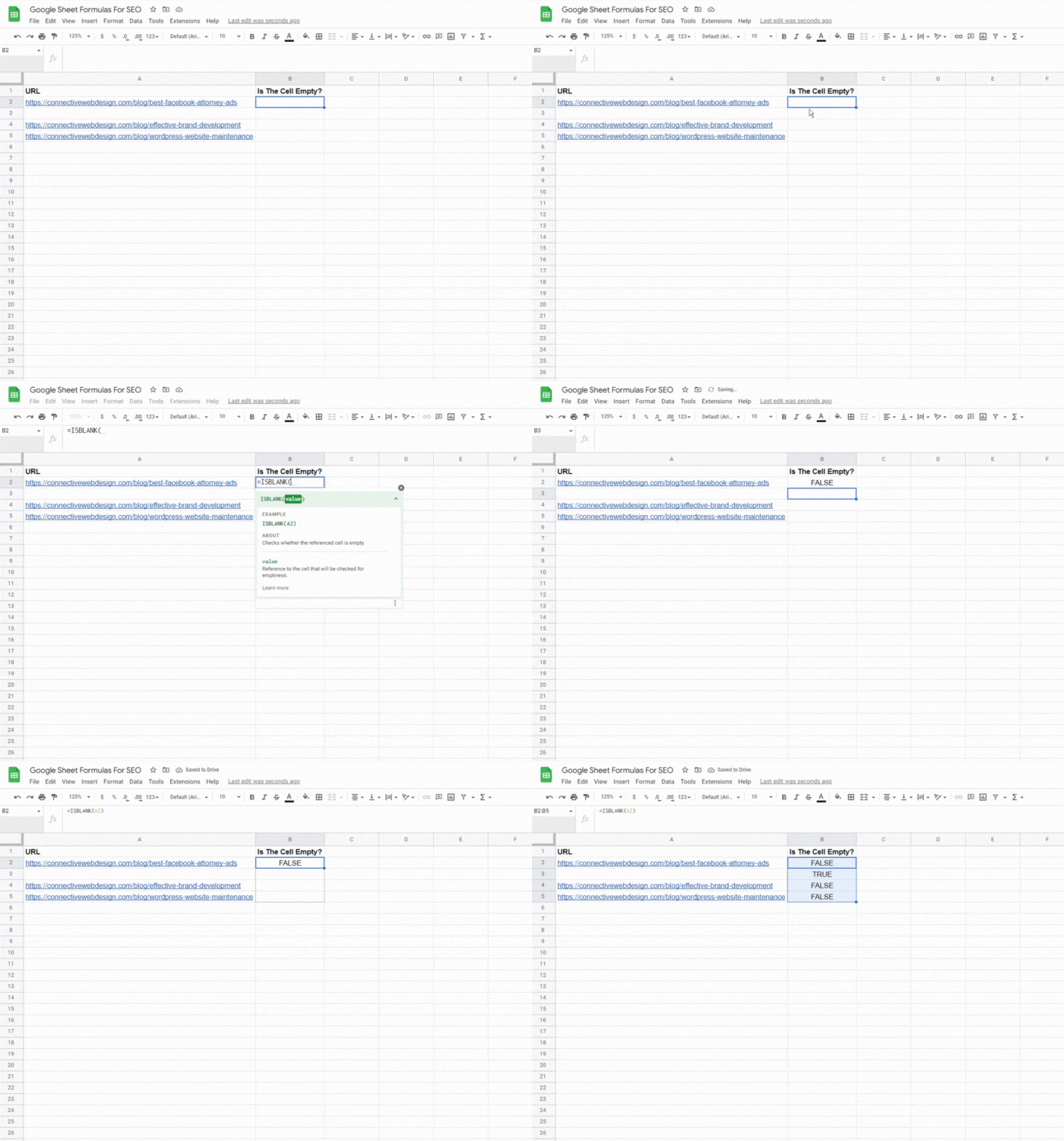
The ISBLANK function checks a cell to determine if it is blank, then returns a TRUE or FALSE value. This function helps you remove regular characters and stray spaces that can affect formula results.
The ISBLANK syntax:
=ISBLANK(cell_reference)
LEN
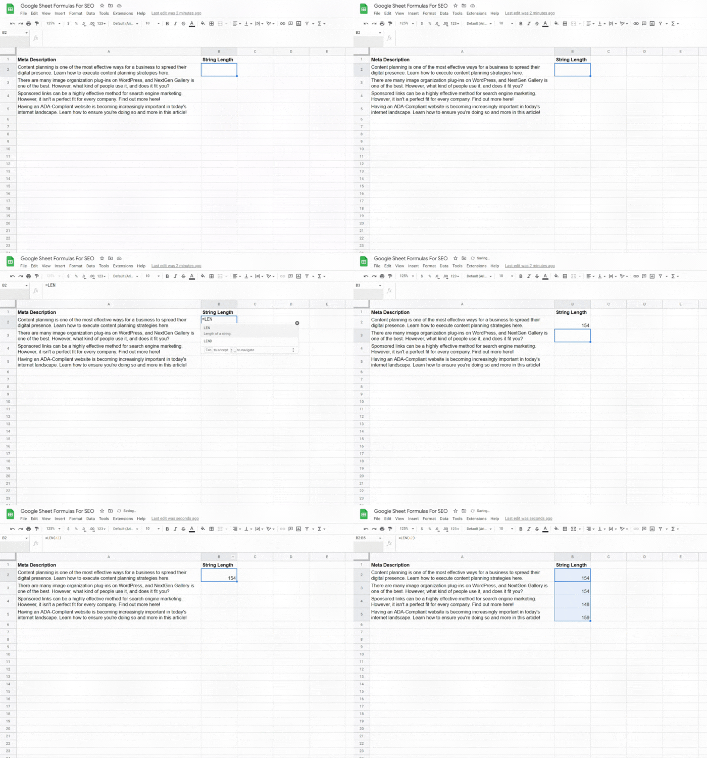
The LEN formula is a popular text function for Google Sheets, and it counts all the characters in a specified string, including spaces, punctuation marks, numbers, letters, and special characters.
This feature is helpful if you need to create page titles or meta descriptions and need to ensure that they have the correct length for Google. For example, your meta title should be under 60 characters.
The LEN syntax:
=LEN(text)
The text argument can either be a direct text value or a cell reference. Consider this example of a LEN function with a direct text value:
=LEN(“Healthy Family – Eco-Friendly Baby Bamboo Toothbrush”)
In this case, the function will return a value of 52 because the text consists of 52 characters, including spaces.
Suppose this title text is in cell A2, and your LEN reference is:
=LEN(A2)
In this case, the LEN function will also return the value of 52.
MATCH
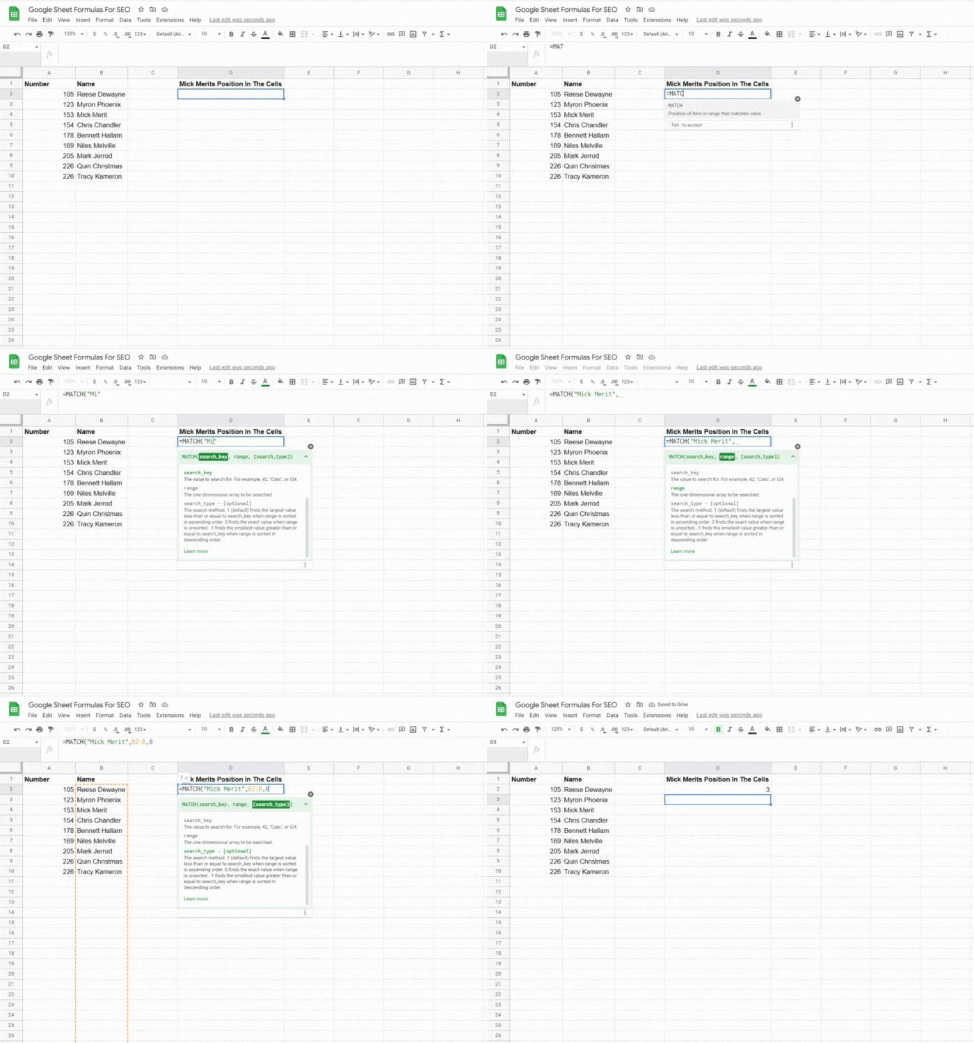
The MATCH function returns the relative position of an item within a range. However, this formula doesn’t return the cell’s value or reference.
For example, if you search for a value, such as a name, that appears fourth in the range, the MATCH function will return a value of “4”.
The MATCH syntax:
=MATCH(search_key, range, search_type)
QUERY
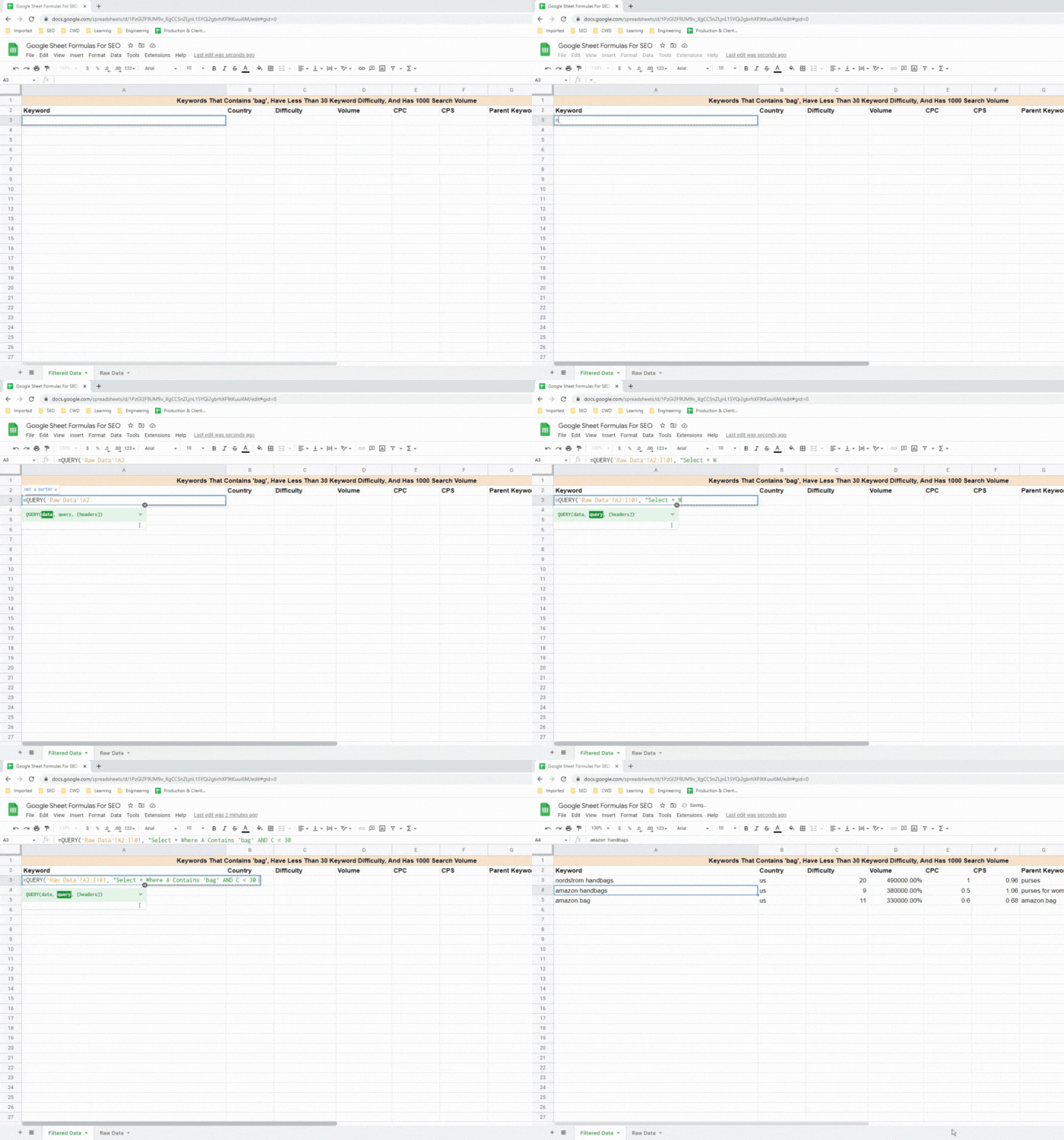
The QUERY function is a powerful tool for changing data in a Google Sheets file. This function also lets you treat all sheets as a database, and you can use it to select statements, import data from one sheet to another, and apply qualifiers to the data you extract.
The QUERY syntax:
=QUERY(data, query, [headers])
The variables in this formula include the range you want to evaluate, the query in quotation marks, and the number of header rows in the data.
REGEX
Regular Expression (REGEX) is a text string you can use to create patterns for matching, locating, and managing text.
Three main REGEX Google Sheets formulas are available:
REGEXEXTRACT
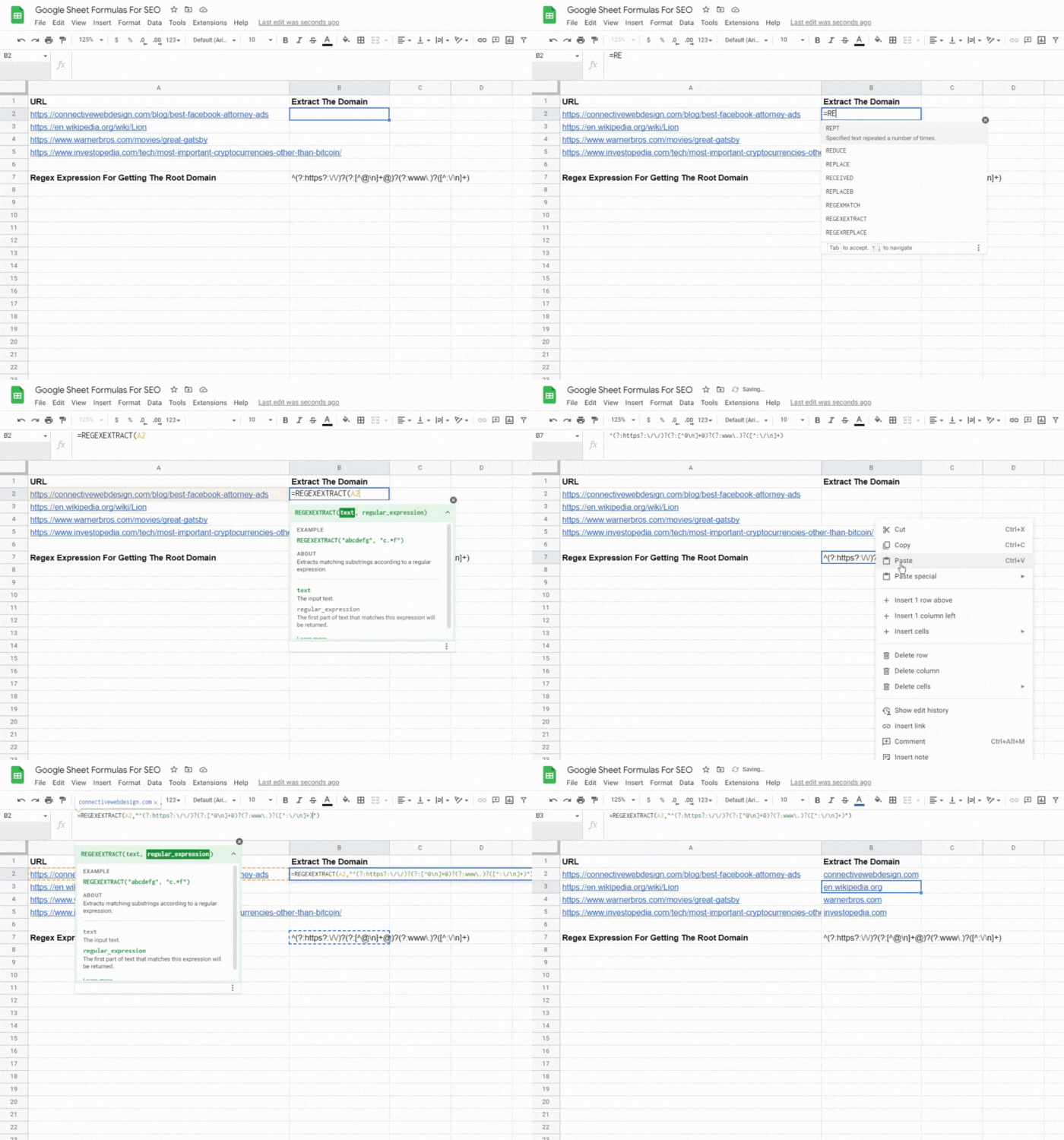
With this formula, you can extract a string from text data. This tool is useful for extracting terms, such as locations, from a list of URLs or keywords.
The REGEXEXTRACT syntax:
=REGEXEXTRACT(text, regular_expression)
REGEXREPLACE
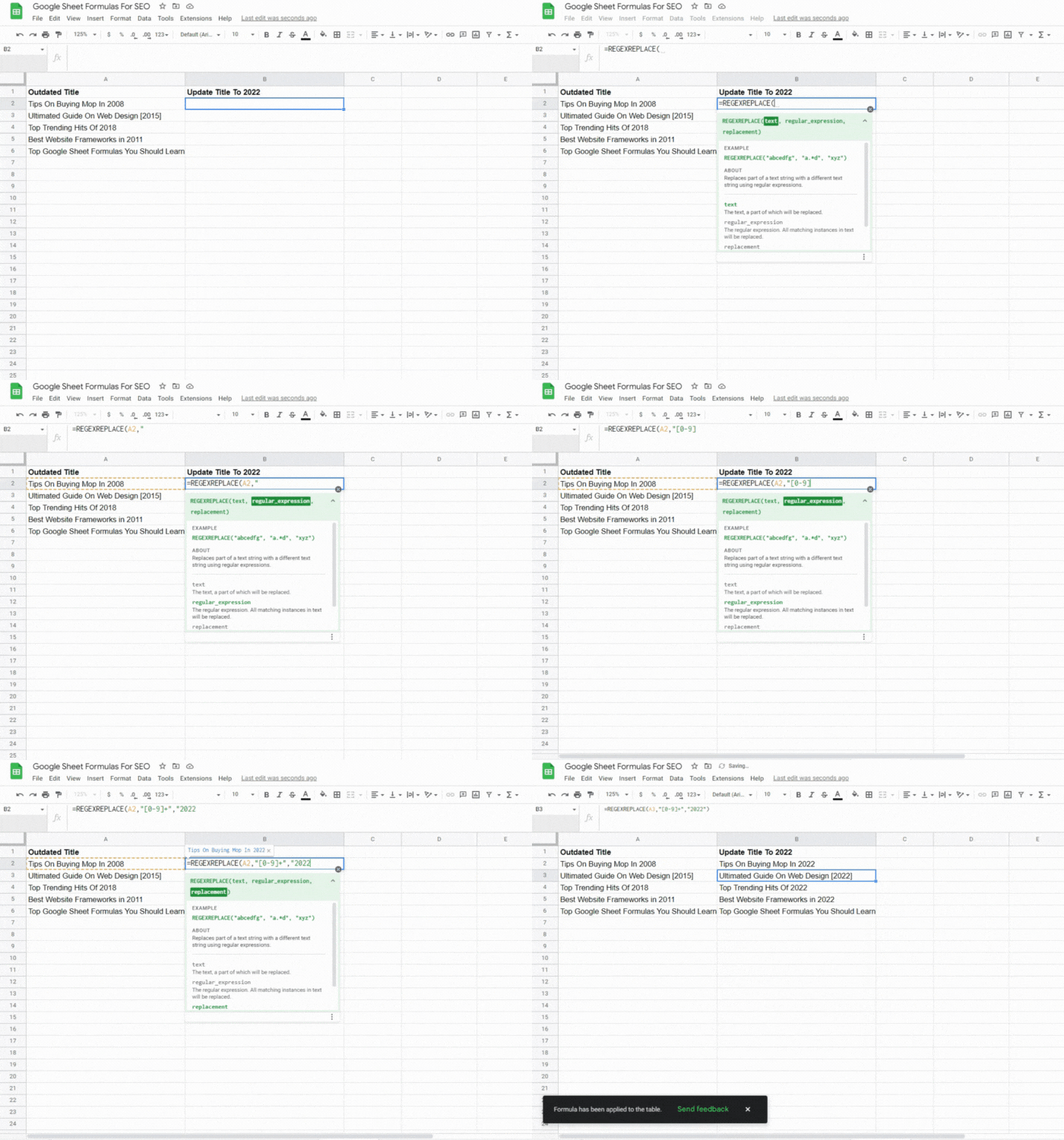
The REGEXREPLACE function lets you replace text in one or more cells using regular expressions. This formula is a handy SEO tool, for example, if you want to capitalize words in a long list of title tags.
The REGEXREPLACE syntax:
=REGEXREPLACE(text, regular_expression, replacement)
REGEXMATCH
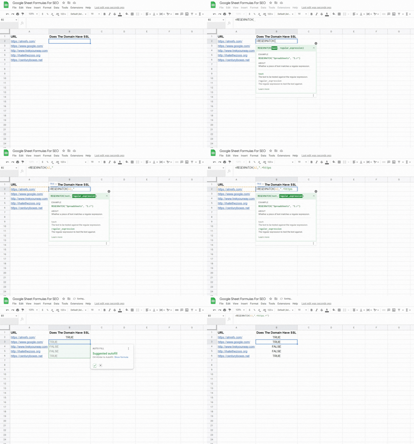
With REGEXMATCH, you can search cell values and return a TRUE or FALSE value depending on a condition. For example, you can use this function to check which URLs in a list contain a specific word.
The REGEXMATCH syntax:
=REGEXMATCH(text, regular_expression)
Unlike REGEXEXTACT, which extracts a text match, REGEXMATCH confirms if a match exists.
SEARCH
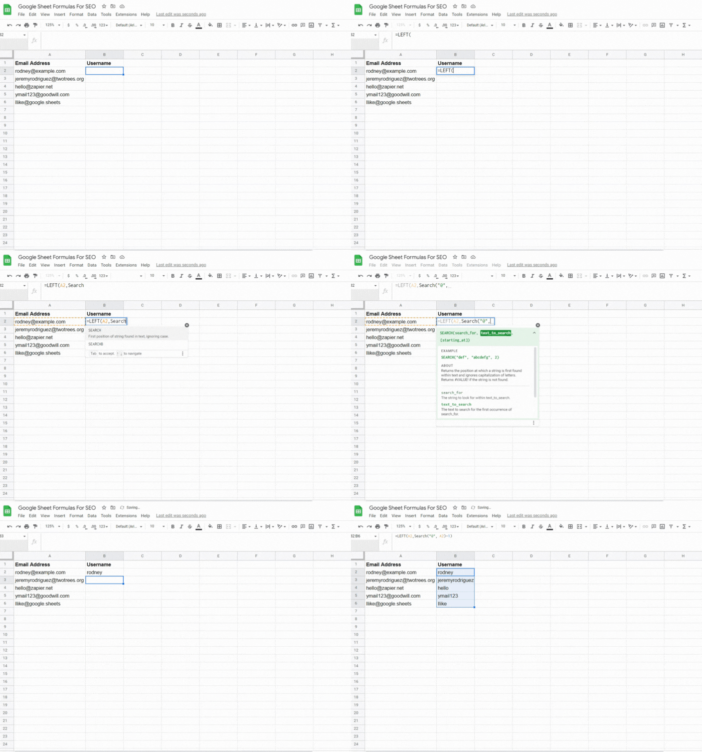
The SEARCH function in Google Sheets lets you locate a substring’s position within a text string.
The SEARCH syntax:
=SEARCH(search_for, text_to_search, [starting_at])
In this formula, search_for is the substring you are looking for, and text_to_search is the main text string containing the substring.
SPLIT
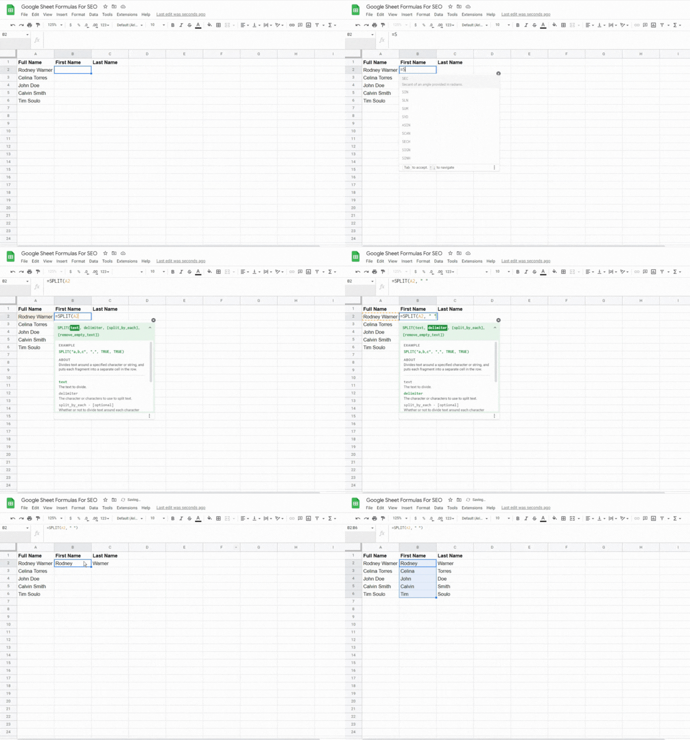
The SPLIT formula in Google Sheets lets you split text-, space-, or comma-separated values into multiple columns.
For example, if you have names and surnames in the same column, you can use this function to split text and create two individual columns: one for names and one for surnames.
The SPLIT syntax:
=SPLIT(text, delimiter, [split_by_each], [remove_empty_text])
In this formula, the text is the cell with the value you want to split. The delimiter is the specific character you want to use to split the text. For example, if you want to split a cell containing “surname, name,” the delimiter is the comma and the space (“, “) between the words.
By default, the split_by_each argument is TRUE, and the function considers each character in the delimiter individually. However, if you don’t want this separate columns function, you need to set the split_by_each argument to FALSE.
By default, the remove_empty_text argument is TRUE, which means the SPLIT function treats multiple adjacent delimiters as one delimiter. If you set this argument to FALSE, this function will add empty cells to the results where you have duplicate delimiters.
SUMIF
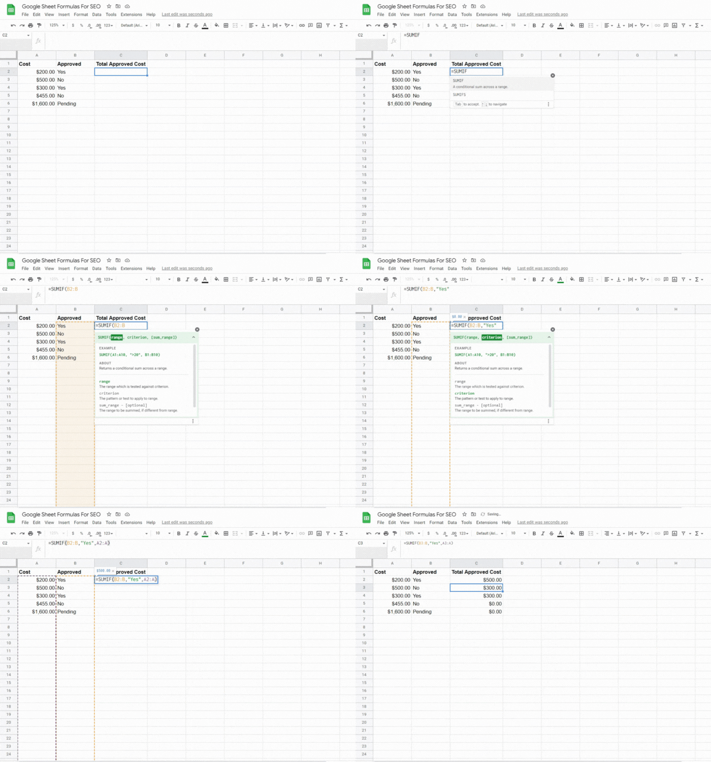
The SUMIF function is not the same formula as the COUNTIF function, but these functions play a similar role. With the SUMIF function, you can tally up the numbers in a Google Sheets range, but only if they meet a certain condition.
The SUMIF syntax:
=SUMIF(range, criterion, [sum_range])
The SUMIF function is helpful if you want to add up traffic according to Google Analytics criteria.
TRIM
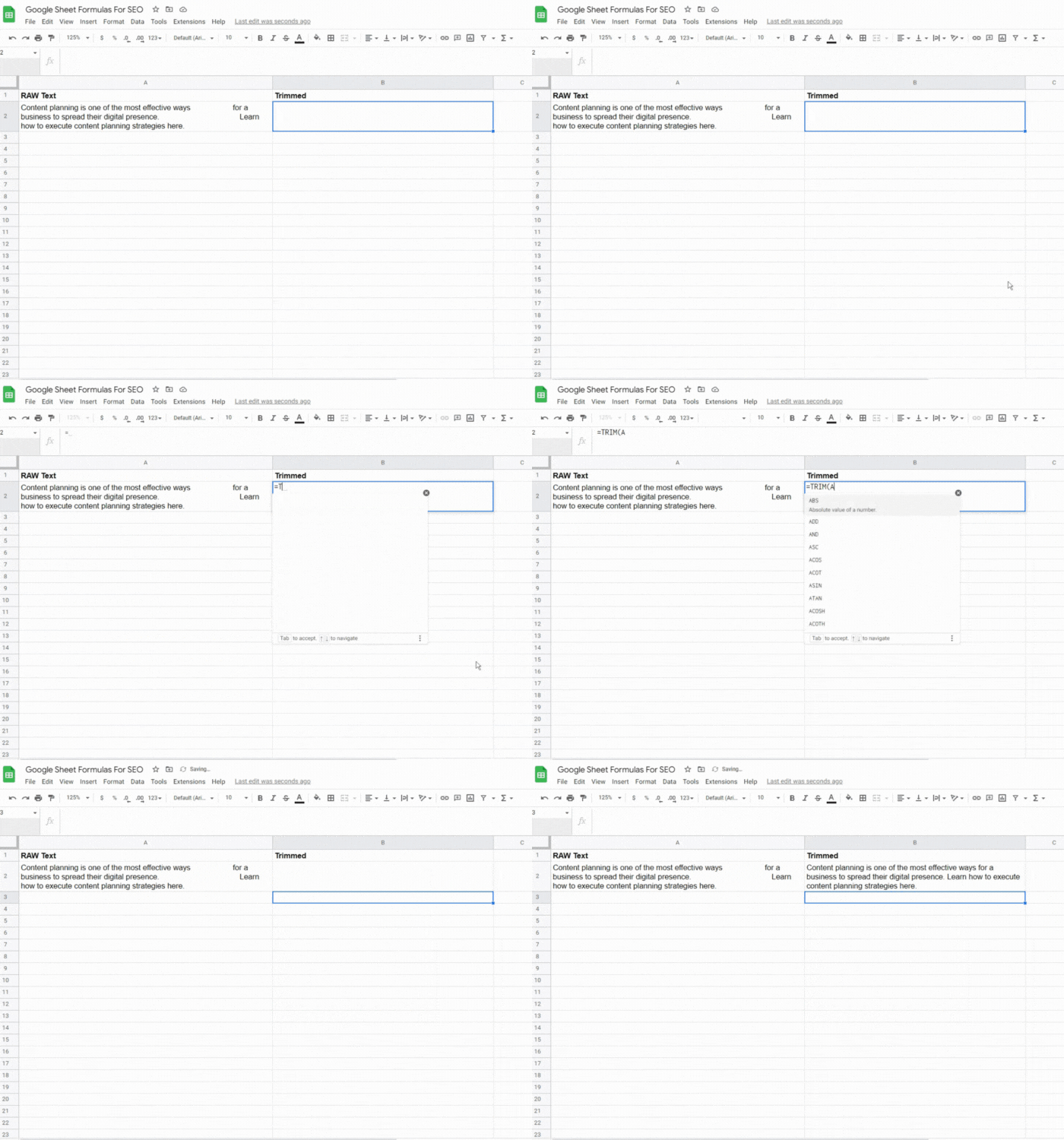
If you import text data into a Google Sheets file, you might end up importing leading and trailing spaces as well, which will affect your formula results. With the TRIM function, you can delete these unwanted spaces, cleaning up your text.
The TRIM syntax:
=TRIM(text)
UNIQUE
The UNIQUE formula provides a convenient way to delete duplicate lines from your data table in a Google Sheets file. In other words, this function only returns the rows that are unique in the source range, and it discards the duplicate data.
The UNIQUE function syntax:
=UNIQUE(range)
This formula is ideal for creating keyword lists without duplication, and it can streamline SEO datasets.
VLOOKUP
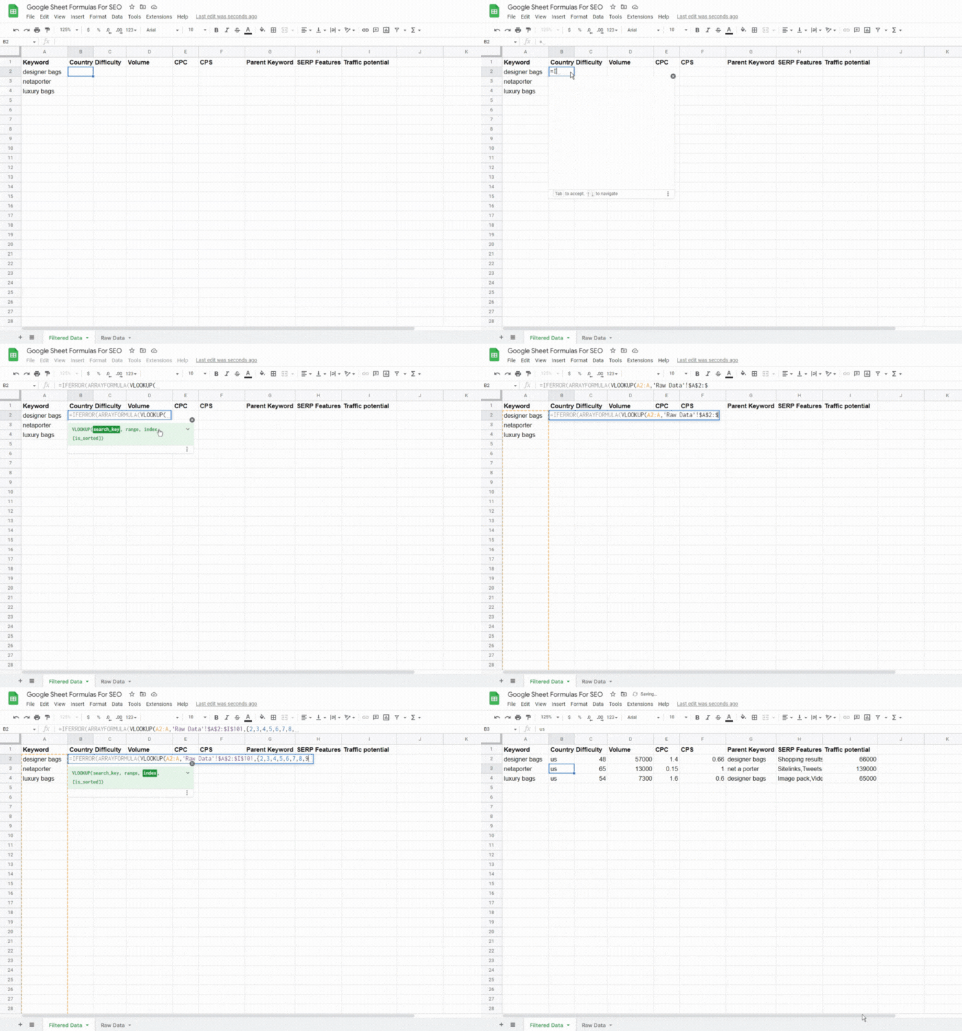
The vertical lookup or VLOOKUP function is a valuable formula for pulling data from one Google sheet into another.
With this formula, you can use a string to search a range and return matching values from one specific cell.
For example, suppose you have two Google sheets: The first sheet (Sheet1) contains a list of keywords with each keyword’s corresponding search volume. The second sheet (Sheet2) features this same list of keywords in column A with each keyword’s corresponding SEO difficulty score in column B.
Using VLOOKUP, you can pull the difficulty scores from Sheet2 and add them to Sheet1.
The VLOOKUP syntax:
=VLOOKUP (search_key, range, index, [is_sorted])
In this formula, the “search key” is the cell containing the common value between the two sheets. In our example, these data points are the keywords.
The range is the worksheet’s name and the relevant columns from where you pull the data. In this example, you want to pull data from Sheet2, the Keyword column (A), and the Difficulty Scores column (B). In the syntax, an exclamation mark must separate the worksheet names and the column range reference.
The index is the column number in the range from where you import data. In this case, the index is 2 because the Difficulty Scores column is the second column in the range.
The is_sorted value indicates whether sorting is necessary (TRUE) or not (FALSE). If no sorting is necessary, the VLOOKUP formula will look for an exact match, which is why we recommend that you set this value to FALSE.
From the above information, you can derive the following formula to pull the difficulty score of the first keyword in cell A2:
=VLOOKUP(A2,Sheet2!A:B,2,FALSE)
Reach out to our team at connective
With the right Google Sheet formulas, you can significantly enhance the effectiveness of your SEO efforts and boost your rankings in the search engine results pages.
If your business needs a comprehensive digital marketing strategy, get in touch with our team at Connective to schedule a strategy session


